Quick Start — 2D wave propagation
This guide builds a minimal but physically meaningful simulation from scratch: monochromatic waves enter a rectangular channel from the left, travel over three Gaussian bumps (shoaling, partial reflection), and are absorbed by a sponge zone on the right.
No Gmsh mesh is required — Tolosa-lct generates the Cartesian grid automatically from the nx, ny, lx, ly parameters. Step 2c shows the equivalent Gmsh mesh if you prefer unstructured grids.
║ ║░░░░░░░░░░░░░ ssh ║ _ _ _ ║░░~sponge~░░░ ~~~ ║______/ \_______/ \________/ \___________║░░░░░░░░░░░░░ ║ ║░░░~60 m~░░░░ West East ssh#user rssh#0.#60.Expected runtime: ~35 seconds on a laptop (sequential, ~25 000 cells).
Prerequisites
Section titled “Prerequisites”- GNU Fortran (
gfortran ≥ 9) or Intel Fortran (ifort) - GNU Make
- ParaView for visualization
1. Clone and compile
Section titled “1. Clone and compile”git clone --recursive https://github.com/TolosaProject/Tolosa-lct.gitcd Tolosa-lctmake C=gnuThe --recursive flag is required to clone the Tolosa-lib submodule. The first make C=gnu compiles — confirm it completes without errors before continuing.
2. Set up your simulation
Section titled “2. Set up your simulation”All files live in bin/. Replace the default input.txt and m_user_data.f90 with the versions below, then recompile.
2a. bin/input.txt
Section titled “2a. bin/input.txt”! ── Cartesian mesh, no Gmsh file needed ──────────────────────nx = 601 ! 300 m / 50 cm per cellny = 41 ! 20 m / 50 cm per celllx = 300. ! domain length [m]ly = 20. ! domain width [m]
! ── Boundary conditions ───────────────────────────────────────bc_N = wallbc_S = wallbc_W = ssh#user ! sinusoidal wave injection via bc_user()bc_E = rssh#0#60 ! 60 m sponge → η = 0
! ── Simulation duration ───────────────────────────────────────simu_time = 5 minutes
! ── Non-hydrostatic splitting ─────────────────────────────────mach = 0.2
! ── VTK output ────────────────────────────────────────────────w_vtk = 11000000 ! basic fields + NH fields (w, p, s_x, s_y)dt_vtk = 1 ! one snapshot per second → 300 frames
! ── Control parameters ────────────────────────────────────────bc_control = wave ! Low-order scheme at bc to stabilizeverbose = 2What the sponge does. rssh#0.#60. relaxes the solution toward η = 0 over the last 60 m of the domain — roughly one wavelength — preventing spurious reflections at the right wall.
2b. bin/m_user_data.f90
Section titled “2b. bin/m_user_data.f90”SUBMODULE (m_Tolosa_lct) m_user_data
implicit none
! ── Wave parameters ────────────────────────────────────────── real(rp), parameter :: A_wave = 0.15_rp ! amplitude [m] real(rp), parameter :: T_wave = 8.0_rp ! period [s]
! ── Background depth ───────────────────────────────────────── real(rp), parameter :: h_bg = 5.0_rp ! [m]
! ── Three Gaussian bumps ───────────────────────────────────── integer, parameter :: nb = 3 real(rp), parameter :: x_bump(nb) = [ 70.0_rp, 155.0_rp, 235.0_rp ] real(rp), parameter :: A_bump(nb) = [ 1.5_rp, 2.0_rp, 1.2_rp ] real(rp), parameter :: sigma_bump(nb) = [ 15.0_rp, 12.0_rp, 18.0_rp ]
CONTAINS
MODULE SUBROUTINE user_parameters( dof , input , mesh ) type(unk), intent(inout) :: dof type(cli), intent(inout) :: input type(msh), intent(inout) :: mesh ! nothing to initialize — all parameters are compile-time constants above END SUBROUTINE user_parameters
MODULE real(rp) FUNCTION bathy_user( x , y ) real(rp), intent(in) :: x , y integer :: i real(rp) :: bump bump = 0._rp do i = 1, nb bump = bump + A_bump(i) * exp( -0.5_rp * ((x - x_bump(i)) / sigma_bump(i))**2 ) end do bathy_user = -h_bg + bump ! positive upward; bumps raise the seafloor END FUNCTION bathy_user
MODULE real(rp) FUNCTION h0_user( x , y , b ) real(rp), intent(in) :: x , y , b h0_user = max( -b , 0._rp ) ! flat free surface at z = 0 END FUNCTION h0_user
MODULE real(rp) FUNCTION u0_user( x , y ) real(rp), intent(in) :: x , y u0_user = 0._rp END FUNCTION u0_user
MODULE real(rp) FUNCTION v0_user( x , y ) real(rp), intent(in) :: x , y v0_user = 0._rp END FUNCTION v0_user
MODULE real(rp) FUNCTION w0_user( x , y ) real(rp), intent(in) :: x , y w0_user = 0._rp END FUNCTION w0_user
MODULE real(rp) FUNCTION p0_user( x , y ) real(rp), intent(in) :: x , y p0_user = 0._rp END FUNCTION p0_user
MODULE real(rp) FUNCTION bc_user( tag , x , y , b ) character(len=*), intent(in) :: tag real(rp) , intent(in), optional :: x , y , b bc_user = A_wave * sin( 2._rp * pi / T_wave * tc ) END FUNCTION bc_user
END SUBMODULE m_user_dataBathymetry explained. bathy_user returns the seafloor elevation (positive upward). With a background depth of 5 m, the flat bottom sits at −5 m. Each Gaussian bump rises above that: the tallest one (2 m at x = 155 m) leaves 3 m of water above it, enough to see clear shoaling without going dry.
Wave injection. bc_user returns η(t) = A sin(2π t / T), which is applied as a prescribed SSH at the West boundary at every time step via the global variable tc (simulation time in seconds).
2c. Alternative: Gmsh mesh (same resolution)
Section titled “2c. Alternative: Gmsh mesh (same resolution)”If you prefer an unstructured mesh — useful for local refinement or irregular boundaries — you can replace the Cartesian nx/ny/lx/ly block with a Gmsh .msh file. The script below reproduces the exact same 300 m × 20 m domain at 0.5 m resolution.
Prerequisites: the Python gmsh package.
pip install gmshbin/domain.py
#!/usr/bin/env python3import gmsh
lx   = 300.   # domain length [m]ly   =  20.   # domain width  [m]size =   0.5  # mesh resolution [m] — same as Cartesian Δx = Δy
gmsh.initialize()gmsh.model.add("domain")
# Corner points: (0,0), (lx,0), (lx,ly), (0,ly)gmsh.model.geo.addPoint(  0,  0, 0, size, 1)gmsh.model.geo.addPoint( lx,  0, 0, size, 2)gmsh.model.geo.addPoint( lx, ly, 0, size, 3)gmsh.model.geo.addPoint(  0, ly, 0, size, 4)
# Boundary linesgmsh.model.geo.addLine(1, 2, 1)   # South (bottom wall)gmsh.model.geo.addLine(2, 3, 2)   # East  (sponge zone)gmsh.model.geo.addLine(3, 4, 3)   # North (top wall)gmsh.model.geo.addLine(4, 1, 4)   # West  (wave injection)
# Surfacegmsh.model.geo.addCurveLoop([1, 2, 3, 4], 1)gmsh.model.geo.addPlaneSurface([1], 1)gmsh.model.geo.synchronize()
# Physical groups — names must match Tolosa-lct BC syntax exactlygmsh.model.addPhysicalGroup(1, [1, 3], 1)gmsh.model.setPhysicalName(1, 1, "wall")       # South + North walls
gmsh.model.addPhysicalGroup(1, [4], 2)gmsh.model.setPhysicalName(1, 2, "ssh#user")   # West: wave injection
gmsh.model.addPhysicalGroup(1, [2], 3)gmsh.model.setPhysicalName(1, 3, "rssh#0#60")  # East: 60 m sponge → η = 0
gmsh.model.addPhysicalGroup(2, [1], 1)gmsh.model.setPhysicalName(2, 1, "surface")
gmsh.model.mesh.generate(2)gmsh.option.setNumber("Mesh.MshFileVersion", 2)gmsh.write("domain.msh")gmsh.finalize()
Run it from bin/:
cd binpython domain.pyThis writes bin/domain.msh (~25 000 triangles). Then replace the Cartesian block in input.txt with:
! ── Gmsh mesh ────────────────────────────────────────────────mesh_name   = domain.msh
! ── BCs are set by physical group names in the .msh file ─────! (bc_N, bc_S, bc_W, bc_E are unused with a Gmsh mesh)
Then recompile and run as before (make C=gnu mrun). The m_user_data.f90 is unchanged — boundary conditions and bathymetry are purely function-based and mesh-agnostic.
3. Compile and run
Section titled “3. Compile and run”make C=gnu mrunThe full output is written to bin/res/run_<timestamp>.txt. On screen you will see:
Startup — mesh and boundary conditions
****************************************************************************************************    _____    _                  _    _   |_   _|__| |___ ___ __ _    | |__| |_     | |/ _ \ / _ (_-</ _` |   | / _|  _|     |_|\___/_\___/__/\__,_|   |_\__|\__|
****************************************************************************************************====================================================================================================* Mesh Loading========================================================================================================================================================================================================* Mesh Loading is OK, with 24000 cells====================================================================================================* - bc tag  1: wall* - bc tag  2: wall* - bc tag  3: ssh is user provided* - bc tag  4: rssh is relaxation zone with length = 6.000E+01 for a fixed ssh = 0.000E+00====================================================================================================* Initialization of relaxation zones done========================================================================================================================================================================================================* Initialize bathy from 'bin/m_user_data.f90'========================================================================================================================================================================================================* Initialize h/u/v/w/p from 'bin/m_user_data.f90'========================================================================================================================================================================================================* SW scheme is switched to dissipative one for h < 10.00 cm========================================================================================================================================================================================================* Dispersion (acoustic) is cutted for h < 0.00 cm========================================================================================================================================================================================================* Maximun acoustic velocity is fixed from Mach number to = 35.02 m/s====================================================================================================
Time loop — one VTK snapshot per second, ~17–18 SW time steps between each:
====================================================================================================* Writing VTK file====================================================================================================nt = 17 t = 3.01890E-01 / 3.00000E+02 ( 0.1 % ) , dt = 1.763611E-02nt = 34 t = 6.00346E-01 / 3.00000E+02 ( 0.2 % ) , dt = 1.751250E-02nt = 52 t = 9.14522E-01 / 3.00000E+02 ( 0.3 % ) , dt = 1.738993E-02...====================================================================================================* Writing VTK file========================================================================================================================================================================================================* Writing restart file (bin)====================================================================================================Profiling table — printed at the end of every run:
**************************************************************************************************** Timer Labels Mean Time (s) Deviation Time (s) Min (s) Max (s) Calls**************************************************************************************************** Time of simulation 3.3660E+01 (100%) 0.0000E+00 ( 0%) 3.366E+01 3.366E+01 1.000E+00 Advance Time 5.2576E-01 ( 2%) 2.4090E-01 ( 1%) 1.200E-05 8.520E-04 3.499E+04 FV Edge Loop (SW) 7.0143E+00 ( 21%) 2.6280E+00 ( 8%) 3.560E-04 1.285E-02 1.750E+04 FV Cell Loop (SW) 1.7590E+00 ( 5%) 4.7842E-01 ( 1%) 8.900E-05 1.845E-03 1.750E+04 FV Edge Loop (AC) 1.3791E+01 ( 41%) 1.0087E+01 ( 30%) 6.500E-05 1.991E-02 1.195E+05 FV Cell Loop (AC) 4.2647E+00 ( 13%) 1.8506E+00 ( 5%) 1.900E-05 7.710E-04 1.195E+05 Cells Detection 7.8421E-01 ( 2%) 1.1702E+00 ( 3%) 9.000E-06 5.594E-03 3.499E+04 Boundary Condition 4.6318E+00 ( 14%) 2.9498E+00 ( 9%) 2.900E-05 6.462E-03 1.370E+05 VTK Output 4.0346E-01 ( 1%) 2.4333E-01 ( 1%) 6.930E-04 1.006E-02 3.000E+02 Savefield 1D Output 1.0550E-03 ( 0%) 4.1649E-03 ( 0%) 0.000E+00 1.000E-06 1.750E+04 Restart (bin) Output 8.0300E-04 ( 0%) 0.0000E+00 ( 0%) 8.030E-04 8.030E-04 1.000E+00 Pre-Treatment 2.5048E-02 ( 0%) 2.9214E-02 ( 0%) 0.000E+00 1.100E-04 1.750E+04**************************************************************************************************** Perf = 8.016E-02 microsec / dx / dt / proc****************************************************************************************************Reading the profiling table. The 24 000 cells come from (nx−1) × (ny−1) = 600 × 40. The time step (~17 ms) is set by the SW CFL at 0.5; the acoustic sub-steps (AC loops) take 38% of total time because NH splitting requires multiple passes per SW step. Boundary conditions account for 13% — normal for a relaxation zone. VTK I/O is cheap at 1%, writing 300 frames total.
VTK files are written to bin/res/vtk/.
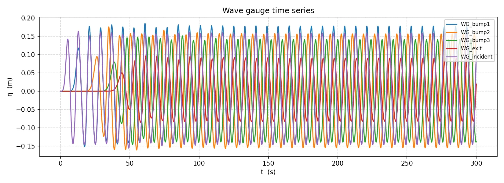
4. Plot gauge time series
Section titled “4. Plot gauge time series”bash bin/finish.shThis reads bin/res/gauge/WG_*.csv and saves bin/gauges.png — one SSH curve per gauge. The five gauges (defined in bin/savefield.yaml) are placed at x = 20, 70, 155, 235, 270 m:
| Gauge | Location |
|---|---|
WG_incident | x = 20 m — flat bottom, incident signal |
WG_bump1 | x = 70 m — above bump 1 (shoaling) |
WG_bump2 | x = 155 m — above bump 2 (tallest, 2 m) |
WG_bump3 | x = 235 m — above bump 3 |
WG_exit | x = 270 m — after bump 3, before sponge |
To add a sub-window VTK output, uncomment the field: block in bin/savefield.yaml.
5. Visualize in ParaView
Section titled “5. Visualize in ParaView”Open the time series
Section titled “Open the time series”- Launch ParaView.
- File → Open — navigate to
bin/res/vtk/. - Select
result_000000.vtk. ParaView detects the sequence and groups all 300 files automatically. - Click Apply in the Properties panel (left side).
Display the free surface
Section titled “Display the free surface”- In the toolbar, open the variable dropdown (initially shows
Solid Color) and selectssh. - Click Rescale to Data Range (circular-arrow icon) to fit the color scale to the wave amplitude.
You should see the channel colored by free-surface elevation, with the three bump locations visible as shallow regions.
Animate
Section titled “Animate”- Click Play (▶) in the time controls at the top.
Watch the wave front travel left to right, deform over the bumps (shoaling and partial reflection), and vanish into the sponge zone at the right.
Next steps
Section titled “Next steps”- Randomize the bumps — move the parameter arrays into
user_parametersand usegenrand(min, max)(from Tolosa-lib) to draw positions and amplitudes at run time. - Add wave breaking — recompile with
make C=gnu SURGE=full ENS=yes mrunand setwave_break_model = 2ininput.txtif any bump brings the water shallow enough for breaking. - Use MPI — for larger grids, add
make MPI=yes extlibonce, thenmake C=gnu MPI=yes NP=4 mrun. - Reference test cases —
tests/wave_in_out_relax/(relaxation BC) andtests/xp-Beji-Battjes/(wave over a bar) are close to this setup and use Gmsh meshes for finer control.