Quick Start — 2D periodic Gaussian forest

This guide runs the default test case shipped in bin/: a 100 m × 100 m periodic domain with 1 000 random Gaussian bathymetric bumps and a random initial free surface. No open boundaries, no forcing — pure free-surface shallow-water dynamics on an unstructured periodic mesh.

     ┌────────────────────────────────┐
  ↕  │  ~  ~  ~  ~  ~  ~  ~  ~  ~  ~  │  ↕
     │  ▲  ▲  ▲   ▲   ▲  ▲  ▲   ▲  ▲  │
     │ _/\_/\_/ \_/ \_/\_/\_/ \_/ \_/ │
     └────────────────────────────────┘
    periodic                      periodic

Expected runtime: ~15 seconds on a laptop (sequential, ~93 000 cells, 2 min simulation).

---

Prerequisites

• GNU Fortran (gfortran ≥ 9) or Intel Fortran (ifort)
• GNU Make
• Python 3 + gmsh for mesh generation
• ParaView for visualization

pip install gmsh

---

1. Clone and compile

git clone --recursive https://github.com/TolosaProject/Tolosa-sw.git
cd Tolosa-sw
make C=gnu PERIO=yes

The --recursive flag is required to clone the Tolosa-lib submodule. PERIO=yes enables the periodic boundary condition support — required for this default case. Confirm compilation completes without errors before continuing.

Note

Change to make C=intel PERIO=yes if you want to use the Intel compiler.

---

2. Generate the mesh

The periodic box mesh is not shipped in the repository (it is regenerated from bin/box.py). Run the provided script once:

bash bin/init.sh

This generates bin/box.msh (~93 000 triangles at 0.5 m resolution) and prints:

Generating box.msh ...
Done — run with: make C=gnu PERIO=yes mrun

Note

After a make superclean, bin/box.msh is deleted. Restore bin/box.py with git restore bin/box.py, then rerun bash bin/init.sh.

---

3. Run

make C=gnu PERIO=yes mrun

Startup — mesh and boundary conditions

****************************************************************************************************
    _____    _
   |_   _|__| |___ ___ __ _   ____ __ __
     | |/ _ \ / _ (_-</ _` | (_-< V  V /
     |_|\___/_\___/__/\__,_| /__/\_/\_/

****************************************************************************************************
====================================================================================================
* Mesh Loading: box.msh
====================================================================================================
====================================================================================================
* Mesh Loading is OK, with 92586 cells
====================================================================================================
* - bc tag  1: periodic
====================================================================================================
* Initialize bathy from 'bin/m_user_data.f90'
====================================================================================================
====================================================================================================
* Initialize h/u/v from 'bin/m_user_data.f90'
====================================================================================================
====================================================================================================
* SW scheme is switched to dissipative one for h < 10.00 cm
====================================================================================================

Time loop — one Tecplot + VTK snapshot per second:

nt =        7 t =  1.35383E-01 /  1.20000E+02 (   0.1 % ) , dt =  1.932828E-02
nt =       13 t =  2.51298E-01 /  1.20000E+02 (   0.2 % ) , dt =  1.931221E-02
nt =       19 t =  3.67077E-01 /  1.20000E+02 (   0.3 % ) , dt =  1.928310E-02
...
nt =     6259 t =  1.20000E+02 /  1.20000E+02 ( 100.0 % ) , dt =  1.121407E-02

Profiling table — printed at the end of every run:

****************************************************************************************************
 Timer Labels               Mean Time (s)       Deviation Time (s)  Min (s)    Max (s)    Calls
****************************************************************************************************
 Time of simulation         1.5650E+01  (100%)  0.0000E+00  (  0%)  1.565E+01  1.565E+01  1.000E+00
 Advance Time               3.4170E-01  (  2%)  3.2462E-02  (  0%)  5.100E-05  1.940E-04  6.259E+03
 FV Edge Loop               1.1913E+01  ( 76%)  1.5003E+00  ( 10%)  1.630E-03  8.398E-03  6.259E+03
 FV Cell Loop               1.3825E+00  (  9%)  8.2170E-02  (  1%)  2.060E-04  6.300E-04  6.259E+03
 Boundary Condition         7.7680E-03  (  0%)  3.7019E-03  (  0%)  0.000E+00  1.500E-05  6.259E+03
 Tecplot       Output       1.8201E-01  (  1%)  2.4167E-02  (  0%)  1.120E-03  2.280E-03  1.200E+02
 VTK           Output       1.2512E-01  (  1%)  1.8806E-02  (  0%)  7.910E-04  1.519E-03  1.200E+02
 Restart (old) Output       5.7700E-03  (  0%)  0.0000E+00  (  0%)  5.770E-03  5.770E-03  1.000E+00
 Restart (bin) Output       1.0580E-03  (  0%)  0.0000E+00  (  0%)  1.058E-03  1.058E-03  1.000E+00
 Pre-Treatment              7.7530E-03  (  0%)  3.5023E-03  (  0%)  0.000E+00  1.800E-05  6.259E+03
 Post-Treatment             1.4169E+00  (  9%)  1.0327E-01  (  1%)  2.140E-04  6.330E-04  6.259E+03
****************************************************************************************************
 Perf = 2.701E-02 microsec / dx / dt / proc
****************************************************************************************************

Reading the profiling table. The FV Edge Loop dominates at 76% — normal for an unstructured mesh with no forcing or open BCs. Post-Treatment (energy, volume) accounts for 9%. The ~6 259 time steps over 120 s give an average Δt ≈ 19 ms, set by the CFL = 0.5 on the 0.5 m cells.

VTK files are written to bin/res/vtk/, Tecplot to bin/res/tecplot/, energy/volume diagnostics to bin/res/.

---

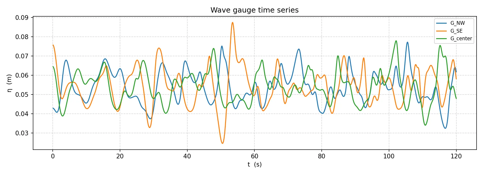
4. Plot gauge time series

bash bin/finish.sh

This reads bin/res/gauge/G_*.csv and saves bin/gauges.png — one SSH curve per gauge. The three gauges (defined in bin/savefield.yaml) cover different locations in the 100 m × 100 m domain:

Gauge	x (m)	y (m)
G_center	50	50
G_NW	20	80
G_SE	80	20

To additionally save a VTK sub-window on the NW quarter, uncomment the field: block in bin/savefield.yaml.

Note

finish.sh requires matplotlib and numpy: pip install matplotlib numpy.

---

5. Visualize in ParaView

Open the time series

1. Launch ParaView.
2. File → Open — navigate to bin/res/vtk/.
3. Select result_000000.vtk. ParaView detects the sequence automatically.
4. Click Apply in the Properties panel.

Display the free surface

5. In the variable dropdown, select ssh.
6. Click Rescale to Data Range to fit the color scale.

You should see the 100 m × 100 m domain colored by free-surface elevation, with the random Gaussian bumps visible as shallow regions.

Animate

7. Click Play (▶) in the time controls.

Watch the free surface evolve as short gravity waves propagate and scatter across the random bathymetry. The periodic boundary conditions make waves re-enter the domain on the opposite side.

Note

To display the bathymetry, open a second render view, load the same dataset, and color it by h (water depth). Shallow cells mark the Gaussian bump crests.

---

Next steps

• Tune the geometry — adjust n_bathy, a_bathy, eps_bathy, h_0 directly in bin/input.txt without recompiling; or edit bin/m_user_data.f90 for structural changes (recompiles at each mrun).
• Add friction — set friction_model = 3 and n = 0.03 in input.txt for Manning friction.
• Use MPI — make MPI=yes extlib once, then make C=gnu PERIO=yes MPI=yes NP=4 mrun.
• Reference test cases — tests/2d_gaussian_forest/ is this exact setup; tests/2d_linear_waves/ is the linear-wave accuracy benchmark.