Tutorial — Wave Breaking on a Slope

This tutorial goes one step beyond the Quick Start: instead of injecting a continuous wave train, you place a solitary wave on a flat bottom, let it shoal up a sloped beach, and capture the breaking event with Tolosa-lct’s enstrophy dissipation model.

The setup reproduces the benchmark of Grilli et al. (1997) — a well-documented FNPM (Fully Nonlinear Potential Model) reference used to validate nearshore wave models.

Expected runtime: ~30 seconds on 6 CPU cores (MPI, ~25 000 cells, ~38 500 time steps).

Reference: Grilli, S. T., Svendsen, I. A., & Subramanya, R. (1997). Breaking criterion and characteristics for solitary waves on slopes. JWPCOE 123(3), 102–112.

---

Prerequisites

Beyond the base requirements from the Quick Start, you need Python 3 with numpy, scipy, matplotlib, vtk, and gmsh:

pip install numpy scipy matplotlib vtk gmsh

---

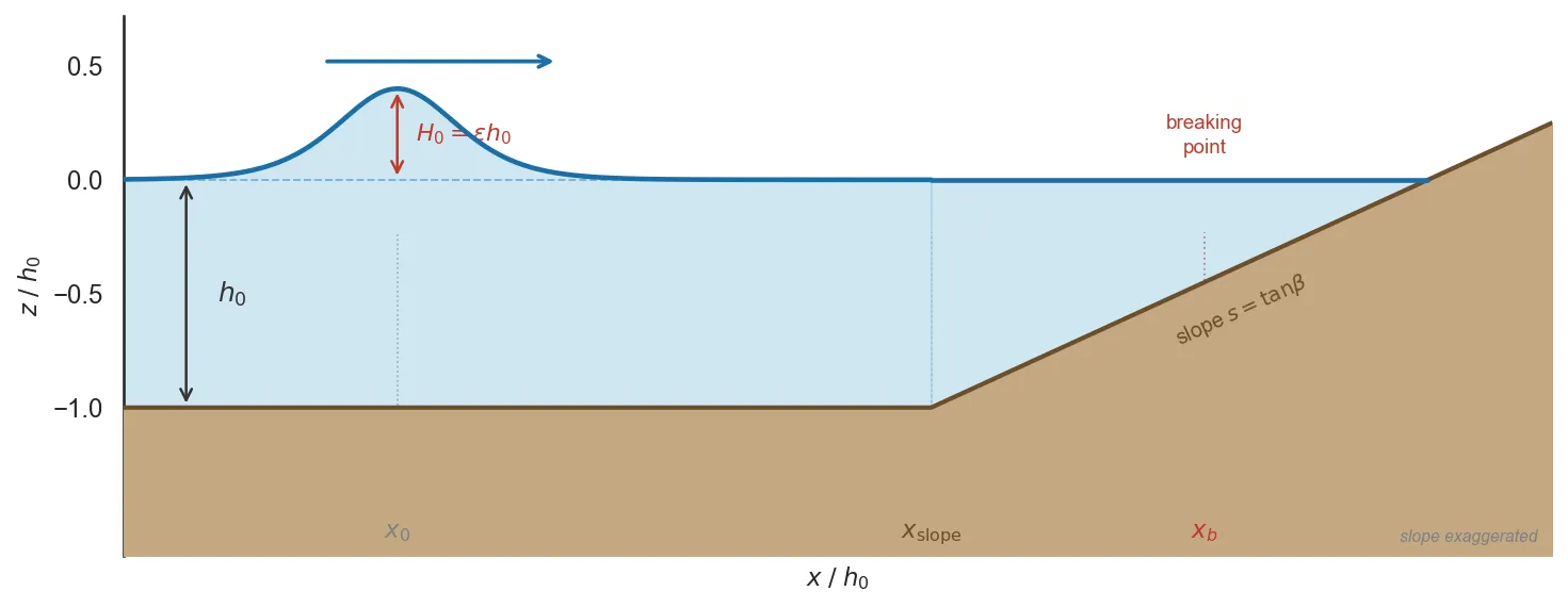
Physics background

A solitary wave of amplitude H₀ on a flat bottom of depth h₀ (ε = H₀/h₀) travels as a coherent structure. When it encounters a slope, it shoals: its height grows and its crest steepens. Past a critical point it breaks.

Grilli et al. measured the breaking location x′_b and breaking height H_b for 9 combinations of slope and amplitude. This tutorial uses case 100_eps40: slope s = 1:100, ε = 0.40 — a Spilling breaker (S₀ = 0.024 < 0.025).

The surf-similarity parameter S₀ classifies the breaking type:

Type	S₀ range	Description
Spilling (SP)	< 0.025	gradual foam on crest
Plunging (PL)	0.025 – 0.30	overturning jet
Surging (SU)	0.30 – 0.37	wave runs up without breaking

The enstrophy model (wave_break_model = 2) detects breaking through the scalar enstrophy ψ and dissipates momentum in the breaking zone. Two parameters control it:

Parameter	Value (slope 1:100)	Role
Re_1	1.7	inverse Reynolds number (dissipation intensity)
psi_0_1	0.08	enstrophy activation threshold

These values are calibrated from Hung (2025, PhD ch. 4.1) against the Grilli data.

---

1. Copy the test case

All files for the Grilli campaign live in tests/surge/grilli/. Copy them to the run directory:

cd Tolosa-lct
cp -r tests/surge/grilli/* bin/

This places in bin/:

File	Role
run_grilli.py	orchestrates mesh, input, run, and plotting for all 9 cases
cnoidal.py	generates the cnoidal/solitary initial wave field
grilli_data/s*.dat	FNPM reference data from Grilli (1997)
m_user_data.f90	bathymetry + initial conditions (slope + solitary wave)
input.txt	default simulation parameters

---

2. Compile with wave breaking support

Wave breaking requires the enstrophy model to be compiled in. The mesh uses periodic BCs (bc_N/S = periodic), so PERIO=yes is also required:

cd Tolosa-lct
make SURGE=scalar PERIO=yes MPI=yes extlib   # compile Scotch partitioner (once)
make SURGE=scalar PERIO=yes MPI=yes C=gnu

Flag	Fields activated	Use case
SURGE=scalar	φ (wave energy) + ψ (enstrophy)	This tutorial — enstrophy breaking
SURGE=scalarw	φ only	Wave energy tracking without breaking
SURGE=full	full tensors φ_ij, ψ_ij	Anisotropic breaking (reference model)

Caution

PERIO=yes is not optional when periodic boundary conditions are used. Omitting it compiles silently but produces wrong results or crashes on any mesh with periodic boundaries.

---

3. Run with run_grilli.py

run_grilli.py handles everything: Gmsh mesh generation, input.txt configuration, soliton initialization, MPI execution, and comparison plotting.

cd bin
python3 run_grilli.py setup run plot --case 100_eps40

The three actions do the following:

setup — creates runs/100_eps40/ with:

• domain.msh — Gmsh mesh (Lx = 124.5 m, dx = 0.05 m, periodic N/S)
• input.txt — configured for s = 1:100, ε = 0.40, ts = 48 s
• run.sh — MPI launch script
• grilli_ref.dat — reference breaking data (x′_b, H_b/h_b, h_b/h₀)

run — calls cnoidal.py to generate the initial soliton field, then launches:

mpirun -np 6 ./exe -s 0.01 -x_slope 20.406 -x0 10.203 -ts 48.0 -dtw 0.480

plot — reads the VTK snapshots, tracks the wave crest position at each frame, and generates runs/100_eps40/100_eps40_compare.png.

Note

The soliton amplitude and mesh size are computed automatically from s and ε by run_grilli.py. The characteristic soliton length L₀ = 1.521/√ε is used to set the initial position and slope distance so the wave has time to establish before reaching the slope.

---

4. Results

Shoaling curve

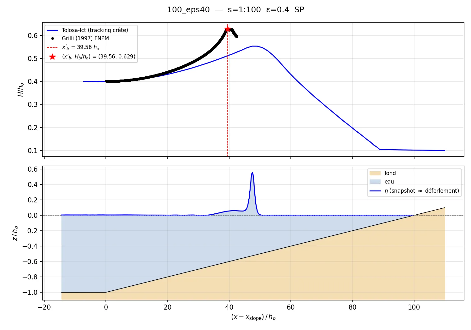
Top panel — H(x)/h₀. The blue curve tracks the spatial crest height at each output frame (VTK snapshot). Black dots are Grilli’s FNPM reference. The two agree well throughout the shoaling phase. The red dashed line marks x′_b = 39.56 h₀ (Grilli breaking point); without the wave breaking model (wave_break_model = 0), Tolosa-lct keeps growing past it — the SGN model captures the steepening but not the post-breaking energy dissipation.

Bottom panel — snapshot near breaking. The free surface (blue) is shown at the frame with maximum crest height. The slope rises from left to right; the sharp spike at x′/h₀ ≈ 47 is the SGN near-breaking structure just before the model diverges.

Breaking-point values for 100_eps40

Quantity	Grilli FNPM	Notes
x′_b / h₀	39.56	distance from slope toe at breaking
h_b / h₀	0.604	water depth at breaking
H_b / h_b	1.041	height-to-depth ratio at breaking

---

5. Key parameters in input.txt

run_grilli.py setup generates a case-specific input.txt. The parameters worth understanding:

! ── Mesh ────────────────────────────────────────────────────
lx = 124.5       ! domain length [m] — flat bottom + slope + margin
ly = 0.5         ! thin channel (quasi-1D)
nx = 2490        ! dx = 0.05 m (20 cells per h₀)
ny = 11

bc_N = periodic  ! thin-channel trick: periodic N/S = quasi-1D
bc_S = periodic
bc_W = wall      ! soliton reflects if it reaches the left wall
bc_E = wall      ! slope extends to the right wall

! ── Time stepping ────────────────────────────────────────────
cfl    = 0.2     ! conservative for the shoaling wave
cfl_ac = 0.8     ! acoustic sub-step CFL
mach   = 0.2     ! acoustic speed = √(gh₀)/mach

! ── Wave breaking ────────────────────────────────────────────
wave_break_model = 0     ! 0 = off, 2 = enstrophy model (Hung 2025)
Re_1             = 1.7   ! calibrated for slope 1:100
psi_0_1          = 0.08

! ── Slope geometry (passed as CLI args to exe) ───────────────
s        = 0.01          ! tan(β) = 1/100
x_slope  = 20.406        ! x-coordinate of slope toe [m]
x0       = 10.203        ! initial soliton crest position [m]
ts       = 48.0          ! simulation duration [s]

Two-run strategy: the setup generates wave_break_model = 0 (off) to see the pure SGN shoaling behaviour and compare with FNPM before the breaking point. To activate the dissipation model, edit runs/100_eps40/input.txt, set wave_break_model = 2, and re-run:

python3 run_grilli.py run plot --case 100_eps40

No recompile is needed — wave_break_model is a runtime parameter.

---

6. What m_user_data.f90 does

Bathymetry — flat bottom at −h₀ = −1 m, then a smooth slope starting at x_slope:

bathy_user = -H_wave + s * 0.5_rp * ( xi + sqrt( xi*xi + r_slope*r_slope ) )

The r_slope term rounds the toe of the slope (radius 0.05 m), avoiding a sharp corner that would generate spurious reflections.

Initial conditions — the soliton profile from cnoidal.bin (written by cnoidal.py) is interpolated onto the mesh. The soliton is centered at x0; the flat-water state (h = h₀, u = 0) is applied outside the soliton footprint.

No boundary injection — bc_user is unused. The soliton is already in the domain at t = 0; there is no wave maker.

---

7. Visualize in ParaView

1. File → Open → runs/100_eps40/res/vtk/ → select result_000000.vtk (series auto-detected).
2. Click Apply.
3. Color by ssh — you’ll see the soliton hump traveling right and growing as it shoals.
4. Switch to psi (enstrophy) — when wave_break_model = 2 is active, the breaking zone lights up as the wave steepens past the threshold.

---

8. Run all 9 cases

Drop --case to run the full 3 × 3 matrix (three slopes × three amplitudes):

python3 run_grilli.py setup run plot

Each case produces its own runs/<name>/<name>_compare.png with the shoaling curve vs FNPM reference. The calibrated breaking parameters per slope (from Hung 2025) are applied automatically.

Case	s	ε	S₀	Type
100_eps20	1:100	0.20	0.0340	PL
100_eps40	1:100	0.40	0.0240	SP
100_eps60	1:100	0.60	0.0196	SP
35_eps20	1:35	0.20	0.0972	PL
35_eps40	1:35	0.40	0.0687	PL
35_eps60	1:35	0.60	0.0561	PL
15_eps30	1:15	0.30	0.1851	PL
15_eps45	1:15	0.45	0.1512	PL
15_eps60	1:15	0.60	0.1309	PL

---

Next steps

• Calibrate for other slopes — change Re_1 / psi_0_1 using the slope-dependent law from Hung (2025):

  Re_1    = 1 + 75 · tan(β)
  psi_0_1 = 0.0909 · (1 + tan(β))^(−30.78) + 0.0123

• Periodic wave breaking — tests/surge/watanabe_perio/ runs a cnoidal wave on a flat periodic domain to validate the enstrophy dissipation rate in a statistically steady state.